CGDSeg — CLIP-Grounded DINOv2
Sclera Segmenter
The sclera is the white, opaque outer shell of the eyeball. It covers about 80% of the eye's surface. Like fingerprints, the blood vessel patterns on the sclera are unique to each person, making it a crucial breakthrough in non-contact biometric identification. Therefore, there is a need for a way to do biometric-pixel-level-precision segmentation of the sclera from eye images.
We use CGDSeg architecture to train two independent Binary Semantic Sclera-Segmentator Models, one of which is trained only on synthetic eye images dataset; while the other is trained on a mix of both synthetic and real eye images dataset.
For Comparison; Our results vastly outperform the winners of last year's International Sclera Segmentation Benchmarking Contest (SSBC 2025) in all categories.
DINOv2-ViT-S/14
21M params
Frozen backbone
Self-supervised
LoRA r=8 α=16
0.59M trainable
QKV adaptation
36:1 compression
CLIP ViT-B/32
63M frozen
Text grounding
4-prompt ensemble
FPN 3-scale
{96,192,384}ch
{64,32,16}px
Param-free upsample
Dense-CSSE
k=32 L=4 blocks
Concurrent attention
3 decoder stages
Output Head
Conv3×3→Conv1×1
Logit threshold 0.5
4ms/image AMP
SynCROI
11,000 pairs
Synthetic eyes
Primary train set
MASD
2,595 real images
3× oversample
Mixed training
SBVPI
1,840 real images
Near-IR sensor
Domain challenge
Navigate with arrow keys, Prev/Next buttons, or the sidetree. 34 slides total.
Problem Formulation
Given an RGB image X ∈ ℝH×W×3, produce a binary mask Ŷ ∈ {0,1}H×W classifying each pixel as sclera or non-sclera. This constitutes a fully convolutional per-pixel binary classification task.
Formal Definition
Challenge Factors
- Substantial intra-class variance: illumination, gaze angle, ethnicity-dependent scleral chromaticity
- Inter-class boundary ambiguity: specular reflections mimic scleral whiteness
- Occlusion by eyelids, eyelashes, and contact lenses
- Synthetic-to-real domain shift between training and test distributions
- Class imbalance: sclera occupies 15–30% of the eye image area
Evaluation Metrics
Competition Context
SSBC 2026 Foundation Model Track mandates the use of a large pre-trained model backbone. Test evaluation is performed on two held-out real-world datasets (MASD, SBVPI) from which the training pipeline has zero samples in the synthetic-only condition.
System Architecture
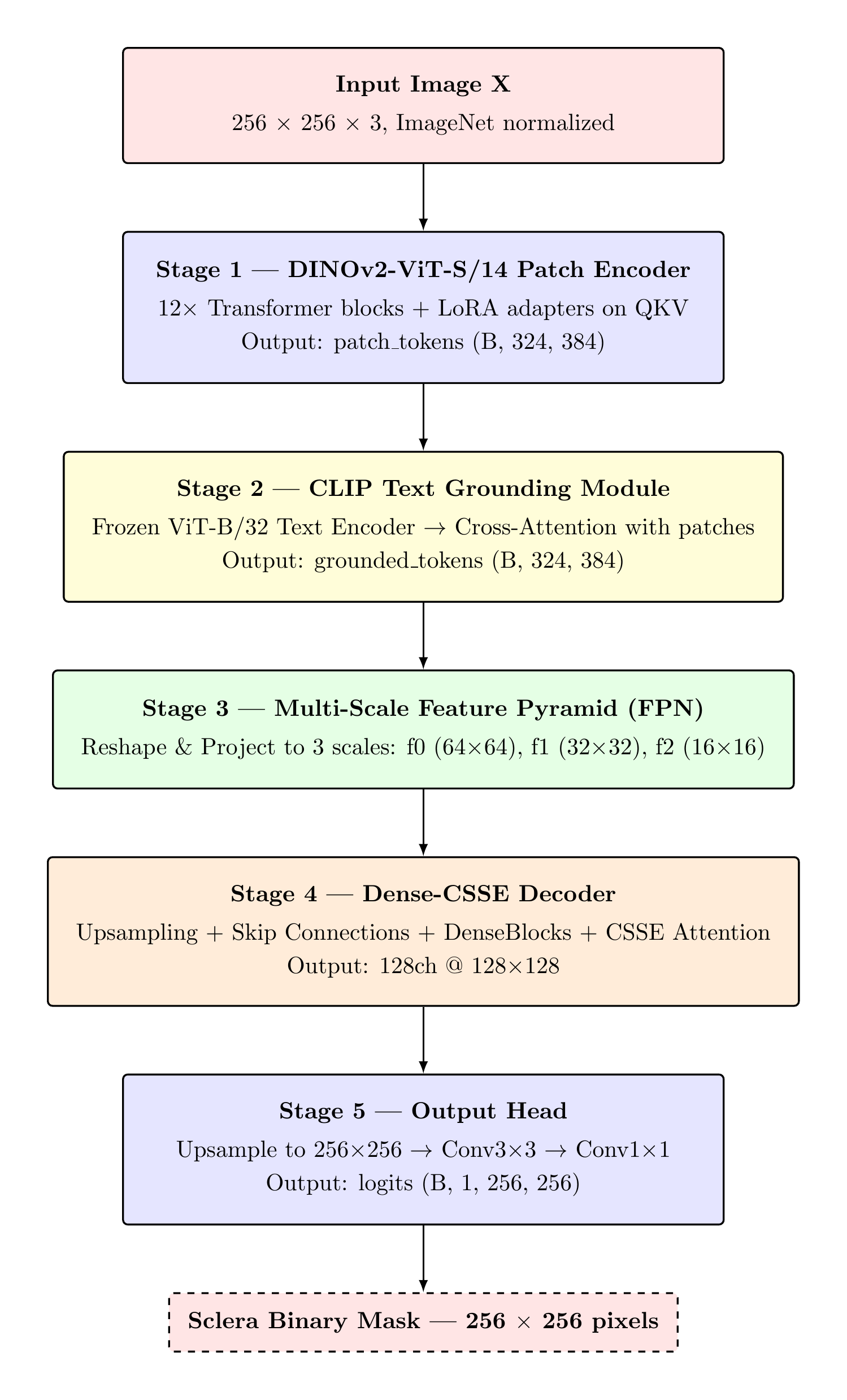
CGDSeg is a five-stage encoder–decoder architecture coupling a frozen pre-trained vision foundation model with a language-grounded cross-attention module and a multi-scale convolutional decoder.
Architectural Philosophy
Parameter efficiency: The two frozen backbones (DINOv2 + CLIP) account for 84.9M of 88.3M total parameters. Trainable capacity is confined to LoRA adapters (0.59M), the CLIP projection and cross-attention (≈0.6M), the FPN projection heads, decoder, and output head (≈2.0M).
Multi-scale decoding: The FPN provides feature representations at 16×16, 32×32, and 64×64 spatial resolutions, enabling the decoder to simultaneously exploit global context and fine-grained boundary information.
Language-guided segmentation: CLIP-based text grounding biases the patch tokens toward semantically relevant sclera features prior to the spatial pyramid, improving disambiguation between sclera and specular highlights.
Parameter Budget Summary
| Component | Params | Status |
|---|---|---|
| DINOv2 ViT-S/14 | 21.0M | Frozen |
| LoRA A,B matrices (×12) | 0.59M | Trained |
| CLIP ViT-B/32 text enc. | 63.1M | Frozen |
| CLIP projection + XAttn | ≈0.60M | Trained |
| FPN proj. heads | ≈0.30M | Trained |
| Dense-CSSE Decoder | ≈1.40M | Trained |
| Output Head | ≈0.30M | Trained |
| Total Trainable | 3.19M | 3.61% |
torch.compile() applied at runtime for kernel fusion and XLA optimisation.
Novel Architectural Contributions
1. Cross-Modal CLIP Grounding in a Segmentation Decoder
Injecting frozen CLIP text embeddings into a pixel-level segmentation backbone via cross-attention is not a standard operation in the segmentation literature. Most CLIP-based segmentation works use CLIP for zero-shot classification of segment proposals (e.g., CLIPSeg, GroupViT), not for modulating the feature representations of a separate vision encoder during training. Here, CLIP acts as a semantic prior injected upstream of the FPN — every pixel-level prediction is implicitly conditioned on the language concept "sclera", even though CLIP never sees the image at inference time. This is a novel use of cross-modal grounding as a regulariser for a domain-specific binary segmentation task.
2. LoRA on ViT Backbone for Ocular Segmentation
Applying LoRA specifically to the QKV projections of a DINOv2 backbone for medical/biometric image segmentation is a key design choice. Unlike NLP LoRA applications where the task distribution shift is often semantic (new domains, styles), the shift here is modality-level: from natural scene photographs to tightly-cropped periocular images with specific illumination conditions. The LoRA rank constraint forces the network to find the minimal spectral direction in weight space that captures the ocular-specific adaptation, effectively learning a "what makes an eye image different from ImageNet" bias without forgetting the rich general-purpose representations. The B=0 initialisation guarantee means the DINOv2 features are perfectly preserved at training epoch 0 — only diverging as evidence accumulates.
3. DenseBlock Decoder for Boundary-Sensitive Segmentation
Standard U-Net decoders use simple Conv→BN→ReLU stacks at each upsampling stage. CGDSeg replaces these with DenseBlocks, providing each decoder convolution with direct access to all prior feature maps within the block. For sclera segmentation, where the target boundary is defined by subtle chrominance and texture gradients (the sclera-iris transition), this dense feature reuse ensures that low-level boundary cues captured early in the block are never discarded — they persist as direct inputs to every subsequent convolutional layer. This is quantitatively significant: the Dec1 DenseBlock input grows from 576 to 704 channels before the transition layer, creating a 128-channel pool of reused features that would otherwise be lost in a standard decoder.
4. Concurrent Channel-Spatial Squeeze-Excitation After Dense Decoding
Placing a CSSEBlock after each DenseBlock+Transition creates a two-stage recalibration: DenseBlock aggregates features through dense connectivity (increasing information richness), then CSSE recalibrates which of those features matter and where. The concurrent (parallel) design of CSSE — where CSE and SSE run simultaneously rather than sequentially — is critical: sequential recalibration would cause the spatial attention to operate on channel-recalibrated features, introducing a dependency between the two attention mechanisms that could limit their complementary roles. Concurrent fusion preserves the independence of "which channels" and "which locations" decisions, allowing them to specialise independently.
5. FPN Without a Separate Encoder Path
Standard Feature Pyramid Networks (Lin et al., 2017) were designed to augment CNN encoders — they top-down combine multi-scale features from different encoder depths. In CGDSeg, there is no multi-scale encoder: DINOv2 outputs a single 18×18 spatial resolution. The FPN here is used purely as a scale constructor — generating multiple resolutions from a single representation via cheap bilinear upsampling and Conv1×1 channel projection. This is a novel adaptation of the FPN concept to the ViT-backbone setting, avoiding the need for intermediate feature extraction from multiple ViT layers (as in multi-scale ViTs like Swin) while still providing the decoder with the spatial diversity it needs for high-resolution mask prediction.
Five-Stage Pipeline
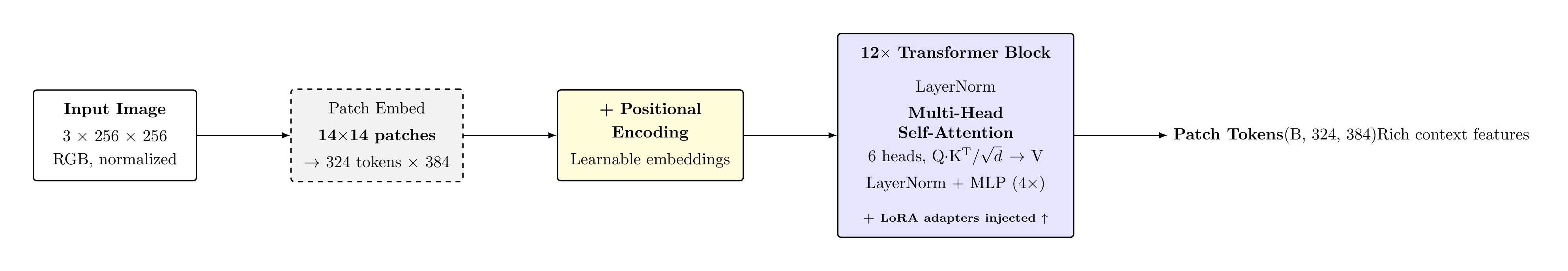
The input image is partitioned into 18×18 = 324 non-overlapping 14×14 patches. A Conv2d(3,384,14,14) patch embedding followed by learnable positional encodings and 12 self-attention Transformer blocks produces a sequence of 384-dimensional contextualised patch tokens. LoRA adapters (r=8, α=16) inject trainable rank-8 perturbations into each block's QKV projections without modifying frozen weights.
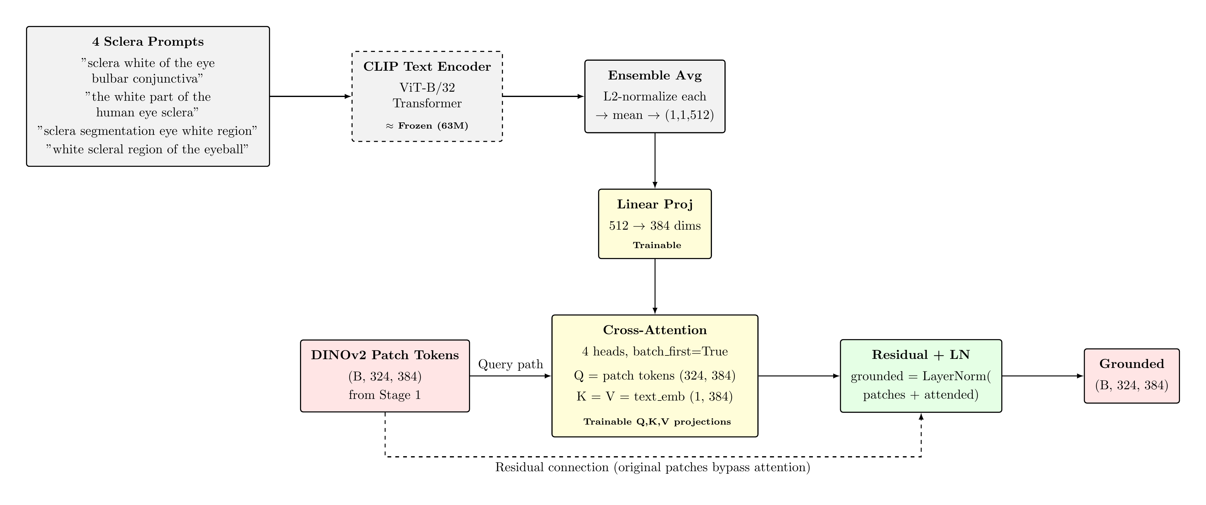
Four sclera-descriptive text prompts are encoded by the frozen CLIP ViT-B/32 text transformer. Resulting embeddings are L2-normalised and averaged into a single 512-dim semantic anchor, which is projected to 384-dim via a trainable linear layer. A 4-head cross-attention module (Q=patch tokens, K=V=text_emb) fuses the text grounding into the visual representation, followed by a residual connection and LayerNorm.
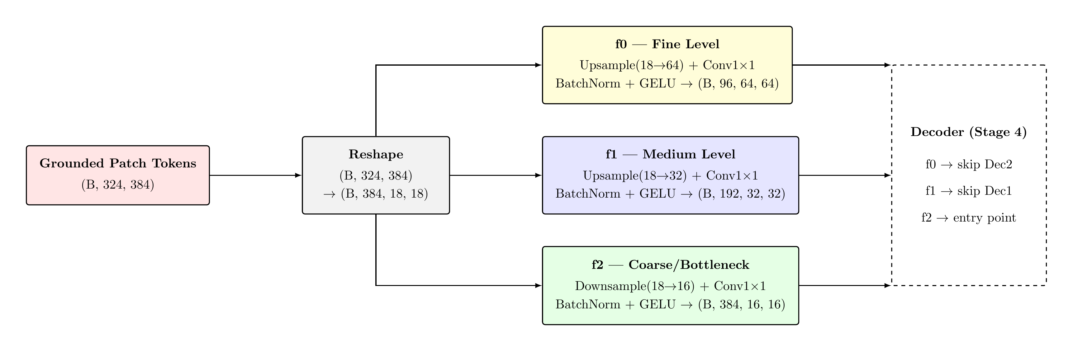
The grounded patch tokens are reshaped into a spatial grid and bilinearly interpolated to three scales. Each level applies a Conv1×1 projection, BatchNorm2d, and GELU activation. Channel widths are chosen as {96, 192, 384} at scales {64, 32, 16} respectively, establishing a standard feature pyramid for the decoder.
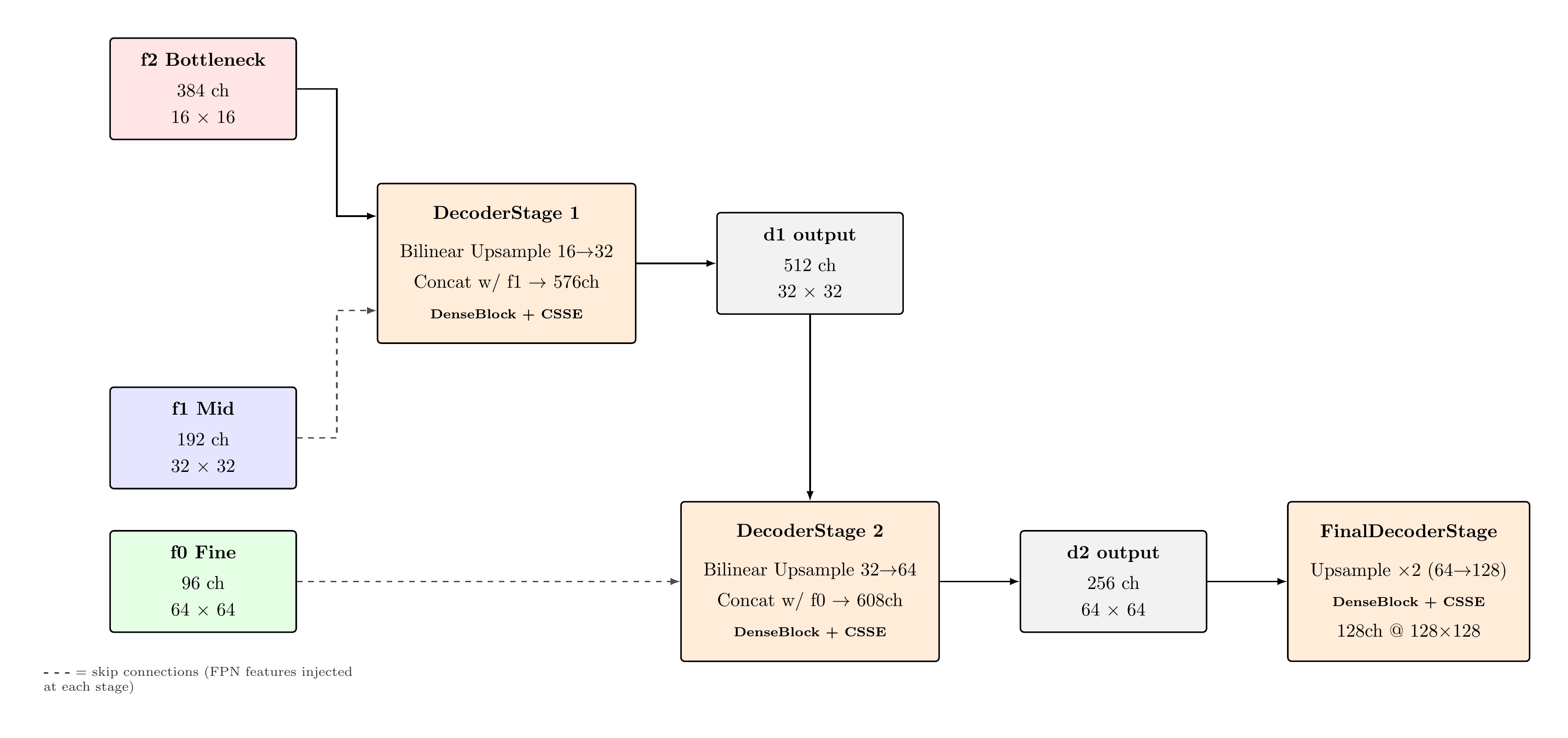
Three progressive upsampling stages reconstruct spatial resolution from 16×16 to 128×128. Each stage concatenates the upsampled feature map with the corresponding FPN skip connection, then applies a DenseBlock (4 layers, growth rate k=32) for dense feature reuse, followed by a CSSEBlock performing concurrent channel and spatial squeeze-excitation recalibration.
Bilinear upsampling restores the feature map to 256×256. A Conv3×3(128→64) with BatchNorm and ReLU provides spatial context aggregation; Conv1×1(64→1) produces the logit map. At inference, σ(logits) ≥ 0.5 yields the binary sclera mask.
Vision Transformer — Architecture & Specifications
DINOv2-ViT-S/14 Specifications
| Attribute | Value |
|---|---|
| Patch size | 14 × 14 px |
| Input resolution | 256 × 256 |
| Spatial grid | 18 × 18 = 324 tokens |
| Embedding dimension d | 384 |
| Transformer blocks L | 12 |
| Attention heads | 6 |
| MLP expansion ratio | 4× (hidden dim 1536) |
| Activation | GELU |
| Dropout | 0.0 (inference) |
| Total parameters | 21M |
| Pre-training | DINO + iBOT on LVD-142M |
| Status in CGDSeg | Frozen |
Why DINOv2 over Supervised ViT?
DINOv2 was trained via self-supervised knowledge distillation (DINO) and masked image modelling (iBOT) on 142M curated images. This yields semantically structured patch representations — patches belonging to the same semantic region exhibit high cosine similarity — without label supervision. Empirically, DINOv2 features generalise to novel tasks with minimal fine-tuning, a critical property given the small sclera segmentation training set.
Position Embedding Resizing
The model's native positional encodings were trained for a 37×37 patch grid (518×518 input). At 256×256 input, the grid reduces to 18×18. The pretrained positional embeddings are bilinearly interpolated from (37,37) to (18,18) grid positions at model load time, as confirmed in the training log:
Rationale for Freezing
Fine-tuning 21M parameters on ≤11,000 training pairs risks catastrophic forgetting of the rich general-purpose representations acquired during large-scale pre-training. The LoRA approach preserves these representations while adapting the model to sclera-specific features through a low-rank perturbation of the QKV projection weights.
Multi-Head Self-Attention
Scaled Dot-Product Attention
Residual Block Structure
Global Receptive Field
Each patch token can attend to all 324 other tokens simultaneously. This is architecturally distinct from CNNs, where receptive field grows logarithmically with depth. For sclera segmentation, this enables a patch at the medial canthus to attend to a patch at the lateral limbus in a single layer — critical for establishing the full extent of the scleral region.
DINOv2 Self-Supervised Pre-training Objectives
| Objective | Description |
|---|---|
| DINO (teacher-student) | Centering + sharpening of softmax distributions between teacher/student views |
| iBOT (masked image) | Token-level masked prediction via soft cross-entropy against teacher |
| KoLeo regularisation | Maximises entropy of patch token distribution across batch |
These objectives collectively encourage patch tokens to encode both local texture and global semantic context — properties directly beneficial to segmentation tasks.
DINOv2 Internal Dataflow
Tensor Dimensions at Each Stage
Low-Rank Adaptation — Mathematical Formulation
Core Formulation (Hu et al., 2022)
Parameter Efficiency
Rank Selection Rationale
Rank r=8 provides sufficient expressivity for domain adaptation from natural images to ocular photographs, consistent with recommendations in the LoRA literature for moderate distribution shift scenarios. Higher ranks (r=16,32) showed marginal improvement in preliminary experiments but substantially increased memory footprint. The rank-8 constraint is not a limitation — it is a deliberate inductive bias: if the difference between DINOv2 features optimised for ImageNet and features optimised for sclera segmentation can be expressed as a rank-8 perturbation, the model is compelled to find the most compact, generalising adaptation.
Alpha Scaling — Why 2.0?
The hyperparameter α=16 with r=8 gives a scale of α/r=2.0. This has a specific interpretation: at initialisation, ΔW=0 (due to B=0), so the first gradient step on A and B is scaled by 2.0 relative to a naive unit-scale LoRA. This accelerates early convergence without destabilising the frozen backbone representations. The choice of α=2r (a common convention) ensures that as r increases, the learning rate contribution per rank dimension remains constant — a desirable invariance property when comparing models across ranks.
Why LoRA Over Other PEFT Methods?
The key insight: The pre-trained DINOv2 weight matrix W₀ encodes a high-dimensional manifold of natural image representations. The adaptation required for sclera segmentation — essentially learning to recognise a specific anatomical region — corresponds to a low-dimensional perturbation of this manifold. LoRA's low-rank constraint directly captures this hypothesis: if the task-specific shift ΔW truly has intrinsically low rank, LoRA will find it exactly; if ΔW is not low-rank, LoRA finds the best low-rank approximation, which is empirically sufficient for most transfer tasks.
LoRA vs. Alternatives
| Method | Trainable Params | Risk |
|---|---|---|
| Full fine-tuning | 21M | Catastrophic forgetting |
| Adapter layers | ~2M | Added latency per block |
| Prefix tuning | ~0.1M | Sequence length sensitivity |
| LoRA r=8 | 0.59M | Low — zero init guarantee |
LoRA Implementation & Injection
LoRALinear Module
Freeze Protocol
Injection Logic
During forward pass, the frozen linear projection and the LoRA bypass are evaluated in parallel and summed. Backpropagation flows only through A and B; W₀ accumulates zero gradient.
total=88.3M params, trainable=3.19M paramsLoRA contributes ≈590K of the 3.19M trainable params.
LoRA Bypass — Visual Architecture
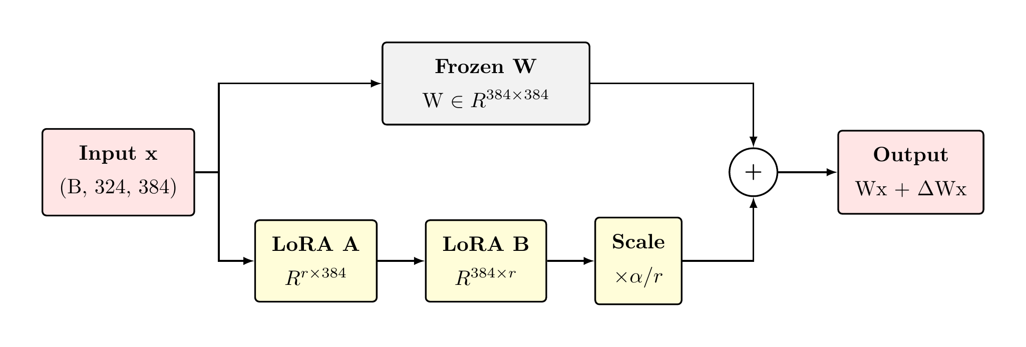
During forward pass, the frozen linear projection (W₀·x) and the LoRA bypass path (B·A·x·α/r) run in parallel and are summed at the output. Only A and B receive gradients — W₀ accumulates zero gradient throughout all 70 training epochs.
total=88.3M params, trainable=3.19M paramsLoRA contributes ≈590K of the 3.19M trainable params.
CLIP Text Encoder & Prompt Ensemble
CLIP ViT-B/32 Text Encoder
| Attribute | Value |
|---|---|
| Architecture | Transformer (12L, 8H) |
| Output dimension | 512 |
| Vocabulary | 49,408 BPE tokens |
| Context length | 77 tokens |
| Parameters | ≈63M (text + image) |
| Pre-training | 400M image-text pairs (OpenAI) |
| Status | Frozen |
Prompt Ensemble
Prompt Ensembling Justification
CLIP text embeddings are sensitive to surface-form prompt variation. The empirical technique of prompt ensembling, introduced alongside CLIP (Radford et al., 2021) and formalised in CoOp (Zhou et al., 2022), averages L2-normalised embeddings of semantically equivalent prompts to produce a more robust, less template-dependent semantic anchor. For sclera, this mitigates the sensitivity to whether the encoder was trained with medical or colloquial descriptions of the structure.
Why CLIP Grounding? — Architectural Innovation
Problem it solves: DINOv2 patch tokens are purely vision-derived — they encode texture, colour, and shape statistics without any semantic alignment to human-defined categories. For sclera segmentation, this means the network must discover the concept "sclera-ness" entirely from visual patterns in the training data, which is particularly challenging given the visual similarity between sclera and specular highlights, or conjunctival vessels near the limbus.
What CLIP contributes: CLIP was trained via contrastive alignment on 400M image-text pairs. Its text encoder maps "sclera white of the eye" to a point in a 512-dimensional semantic space where visually similar concepts cluster together. By projecting this semantic anchor into the patch token space and fusing it via cross-attention, we impose a learned semantic bias on the patch token sequence — patches representing the scleral region are pulled toward this anchor, while patches representing non-sclera structures are not.
Zero-cost at inference: The text embedding is computed once and cached. At training and inference time, CLIP contributes zero FLOPs beyond the single cached matrix multiply in the projection layer and the cross-attention operation. This is fundamentally different from approaches that require joint vision-language processing per image.
Integration into Forward Pass
Cross-Attention Grounding Mechanism
Self- vs. Cross-Attention
Self-attention (used in DINOv2 internally) computes queries, keys, and values from the same token sequence. Cross-attention draws queries from one sequence (patch tokens) and keys/values from another (text embedding), enabling inter-modal information fusion without altering the query sequence's positional structure.
Attention Score Interpretation
Feature Pyramid Network
Motivation for Multi-Scale Representation
A single-resolution feature map at 18×18 pixels (the DINOv2 output) is insufficient for high-quality boundary delineation at 256×256 target resolution. The FPN constructs a set of feature maps at progressively finer spatial resolutions while reducing channel depth, providing the decoder with both high-level semantic information and spatial precision at each upsampling stage.
Scale Construction
Design Decisions
Channel halving: Channel widths {384, 192, 96} follow a 2× reduction per scale level, balancing computational cost against feature capacity. Finer scales carry lower channel depth because spatial information compensates for reduced representational dimensionality.
GELU activation: GELU is used in the FPN projection heads for consistency with DINOv2 and CLIP's internal activations. Activation consistency across stages reduces representational mismatch at the feature boundaries.
Bilinear interpolation: Bilinear upsampling from 18×18 to each target resolution is artifact-free and parameter-free. The Conv1×1 projection following the upsample provides the learnable channel mixing necessary for scale-appropriate feature extraction.
Why FPN Over U-Net Encoder?
The architectural insight: A classical U-Net requires a dedicated encoder path that progressively downsamples the input image, storing skip connections at each resolution. With DINOv2 as the backbone, this entire encoder is already provided — the 12-block ViT outputs patch tokens that already encode multi-level semantic information through its depth. Building a separate encoder on top of DINOv2 would be redundant and computationally expensive.
What the FPN does instead: Rather than encoding multiple input resolutions, the FPN decodes a single, rich 18×18 representation into multiple spatial scales via cheap bilinear interpolation and Conv1×1 channel projection. This is O(C) cost per scale level, versus O(H²·C) for a full convolutional encoder path — an enormous computational saving that contributes directly to the 3.61% trainable parameter fraction.
The bottleneck asymmetry: Notably, f2 (the coarsest FPN scale) performs a slight downsampling from 18×18 to 16×16. This produces a clean 2× spatial relationship across all three scales (16→32→64), simplifying the decoder upsampling arithmetic and avoiding misaligned concatenation at decoder stages.
| Level | Spatial | Channels | Semantic Level |
|---|---|---|---|
| f2 | 16×16 | 384 | Global / bottleneck |
| f1 | 32×32 | 192 | Mid-range context |
| f0 | 64×64 | 96 | Spatial / boundary |
FPN Dataflow
FPN vs. U-Net Skip Connections
Unlike a standard U-Net encoder–decoder, which must pass information through all intermediate layers before generating skip connections, the FPN creates skip features directly from the ViT output representation, independently processed at each scale. This avoids the spatial degradation that occurs when skip information must flow through multiple downsampling operations.
DenseBlock — Architecture & Dense Connectivity
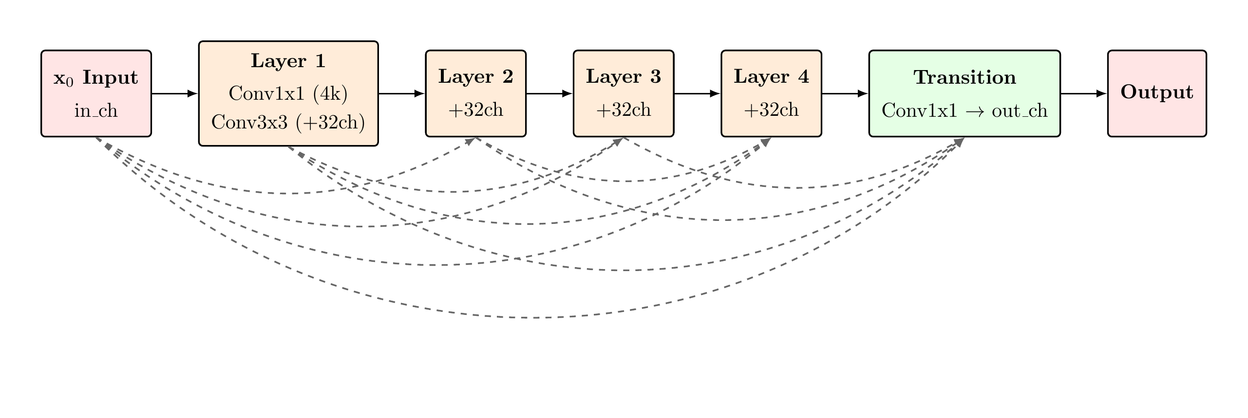
DenseNet Layer (Huang et al., 2017)
In a DenseBlock with L=4 layers and growth rate k=32, the input to layer ℓ is the concatenation of all prior layer outputs:
Dense Connectivity — Full Skip Connection Map
Advantages of Dense Connectivity
- Implicit deep supervision: Loss gradients propagate directly to all preceding layers, mitigating vanishing gradient in the decoder. Each layer receives direct gradient signal from the final loss, effectively acting as if it were the last layer — this is particularly valuable in narrow decoder pathways where gradient flow might otherwise degrade.
- Feature reuse without redundancy: Each layer has direct access to all antecedent feature maps. Unlike ResNets (which add features), DenseBlocks concatenate them — the network can learn to select from the full feature history, exploiting low-level edge detectors and high-level semantic activations simultaneously at each stage.
- Regularisation through diversity: Concatenating L prior feature maps at each layer input forces the subsequent convolutional kernel to operate on a highly heterogeneous input manifold. This implicit diversity serves as a regulariser analogous to dropout — overfitting to any single feature map is structurally penalised.
- Parameter efficiency: Dense connectivity achieves high effective depth with fewer parameters per layer. A standard 4-layer block with growth rate k=32 adds only 4×32=128 channels while providing 10 total connection paths — far richer connectivity than a plain 4-layer stack of equivalent width.
- Bottleneck + transition compression: The 4k bottleneck (Conv1×1→Conv3×3) pattern and final transition Conv1×1 provide channel compression that prevents quadratic channel explosion, keeping memory cost tractable even with dense concatenation.
Why DenseBlock in This Decoder?
The sclera boundary is defined by extremely subtle texture gradients — at 256×256, the sclera-iris boundary is often 1–2 pixels wide. Standard decoder layers (simple Conv→BN→ReLU stacks) risk discarding fine-grained boundary evidence as features propagate through the upsampling stack. DenseBlocks preserve this evidence by keeping all intermediate feature maps accessible at every layer, making it particularly well-suited to boundary-sensitive segmentation tasks. The growth rate k=32 is deliberately conservative — it allows the network to accumulate boundary-relevant features without overwhelming the semantic context features carried from the FPN.
Channel Accounting per Decoder Stage
| Stage | Input (after cat) | DenseBlock Out | After Trans. |
|---|---|---|---|
| Dec1 | 384+192=576 | 576+128=704 | 512 |
| Dec2 | 512+96=608 | 608+128=736 | 256 |
| Dec3 | 256 (no cat) | 256+128=384 | 128 |
CSSEBlock — Channel & Spatial Squeeze-Excitation
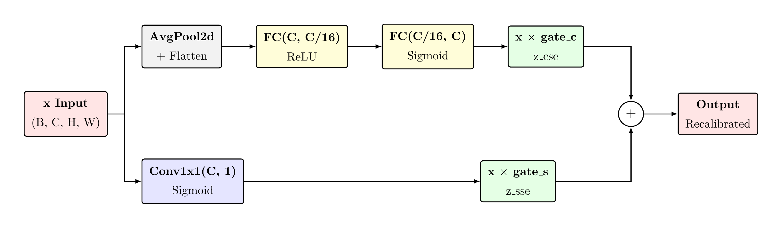
Channel Squeeze-Excitation (CSE) — In Depth
Spatial Squeeze-Excitation (SSE) — In Depth
Concurrent Fusion — Design Rationale
CSE vs. SSE: Complementary Roles
CSE addresses which features are informative: the global average pooling aggregates spatial context into a channel descriptor, and the bottleneck FC network learns channel interdependencies. For sclera segmentation, CSE can suppress chrominance features and amplify edge-sensitive channels.
SSE addresses where in the feature map to focus: the spatial attention map identifies regions of high relevance, providing a form of spatial gating independent of channel composition.
CSSEBlock — Concurrent Squeeze-Excitation Architecture
The CSSEBlock applies channel and spatial squeeze-excitation in parallel, independently recalibrating both "which features matter" (CSE) and "where features matter" (SSE), then summing their outputs for dual recalibration.
Decoder Progressive Upsampling
Output Head & Inference
Head Architecture
Design Rationale
Bilinear head upsample: Restores the 128×128 decoder output to the 256×256 input resolution. Bilinear interpolation is preferred over transposed convolution to avoid checkerboard artifacts at this final stage.
Conv3×3 before Conv1×1: The 3×3 convolution aggregates a local spatial context prior to the binary classification projection, providing a spatially-aware feature vector at each pixel location as opposed to a purely point-wise prediction.
Logit loss vs. probability loss: The binary cross-entropy is computed on raw logits via
F.binary_cross_entropy_with_logits, which computes the sigmoid internally using the
numerically stable log-sum-exp formulation, avoiding floating-point underflow at extreme probability
values.
Logits: (B, 1, 256, 256) float32
Probs σ(): (B, 1, 256, 256) ∈ [0,1]
Binary mask: (B, 1, 256, 256) ∈ {0,1}
SSBC submit: upsampled to 400×300
Forward Pass — Complete Shape Trace
Complete System Flowchart
Loss Function — DiceBCE Formulation
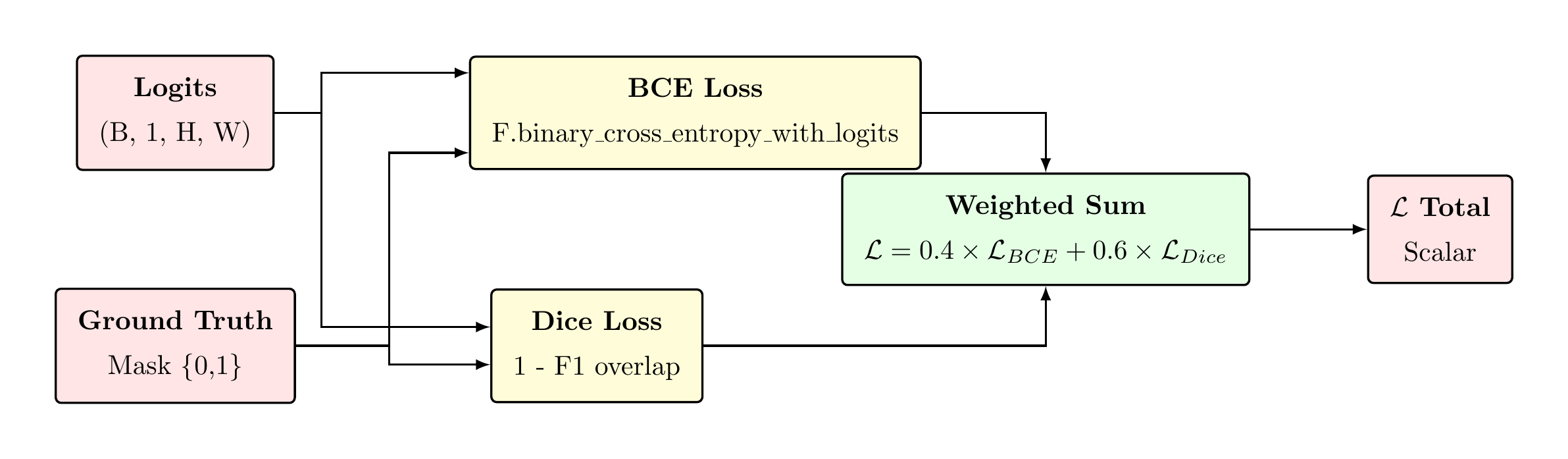
Binary Cross-Entropy Component
Soft Dice Loss Component
BCE provides dense per-pixel gradient signal, enabling rapid early-epoch convergence. Dice focuses on region overlap, providing class-balanced supervision that is robust to the sclera/background imbalance. The 0.4/0.6 split was determined empirically to prioritise region overlap while retaining per-pixel precision.
Optimizer, Learning Rate, & Schedule
AdamW Optimizer
Cosine Annealing Schedule
LR Trajectory Chart
Rationale for Differential LR
LoRA parameters require a lower learning rate than the task-specific modules (FPN, decoder, head) because they modify the representations of a frozen, pre-trained backbone. A larger LoRA learning rate risks over-steering the QKV projection perturbations, degrading the DINOv2 representations.
Data Augmentation Pipeline
Geometric Transforms
| Transform | Probability | Parameters |
|---|---|---|
| Horizontal flip | p=0.50 | — |
| Vertical flip | p=0.30 | — |
| Affine rotation | p=0.40 | θ ∈ [−15°, 15°] |
| 90° rotation (k) | p=0.15 | k ∈ {1,2,3} |
Photometric Transforms
| Transform | Probability | Parameters |
|---|---|---|
| Brightness/contrast | p=0.60 | α∈[0.8,1.2], β∈[−30,30] |
| HSV hue/saturation | p=0.40 | Δhue∈[−18,18], sat×[0.7,1.3] |
| Gaussian noise | p=0.30 | σ∈[5,20] |
| Gaussian/motion blur | p=0.25 | σ∈[0.5,3.0] |
| JPEG compression | p=0.25 | Q∈[30,95] |
Occlusion Augmentation
| Transform | Probability | Parameters |
|---|---|---|
| Random rectangles | p=0.40 | 0–3 rects, variable size |
| Specular highlights | p=0.25 | 1–3 Gaussian blobs, s∈[0.3,0.8] |
Implementation Notes
Geometric consistency: All geometric transforms are applied identically to the image and
its corresponding binary mask using the same random parameters (enforced via shared
random.random() seeds per sample), preserving pixel-level annotation validity.
Specular highlight simulation: The specular augmentation adds Gaussian-shaped intensity blobs to the image only (not the mask), specifically simulating corneal and scleral specular reflections that constitute a primary source of false positives for sclera detection.
Dataset Composition
Dataset Summary
| Dataset | Type | Pairs | Use |
|---|---|---|---|
| SynCROI | Synthetic | 11,000 | Train/Val |
| MASD | Real (photographs) | 2,595 | Train (mixed) / Test |
| SBVPI | Real (photographs) | 1,840 | Train (mixed) / Test |
| Total | — | 15,435 | — |
Cache Statistics (from log)
Dataset Bar Chart
SynCROI Train/Val Split
Mixed Training Strategy
Rationale
In the synthetic-only condition, the model trains and validates on SynCROI, exhibiting strong in-domain performance (val F1 = 0.9771) but reduced cross-domain generalisation (MASD test F1 = 0.8795). The synthetic-to-real domain gap arises from differences in illumination distribution, lens characteristics, and scleral texture between rendered and photographic images.
The mixed strategy incorporates real-world images during training, directly exposing the model to the target domain distribution and substantially improving real-world test performance.
Mixed Dataset Composition
Oversampling Design
Real images are oversampled at 3× to counteract the numerical dominance of the synthetic dataset. Without oversampling, real images would constitute only ≈30% of each epoch's training distribution, insufficient to overcome the domain prior established by the synthetic data. The 3× factor balances domain representation while retaining the synthetic data's annotation density advantage.
Mixed vs. Synthetic Comparison
| Metric | Synthetic | Mixed | Δ |
|---|---|---|---|
| Val F1 (SynCROI) | 0.9771 | 0.9729 | −0.0042 |
| MASD Test F1 | 0.8795 | 0.9546 | +0.0751 |
| SBVPI Test F1 | 0.8664 | 0.9336 | +0.0672 |
The mixed model incurs a marginal 0.42pp drop on in-domain validation, which is expected due to the increased distribution complexity. The gains on real-world test sets (+7.5pp, +6.7pp) substantially outweigh this trade-off.
Training Curves — Mixed Model
Convergence Characteristics
The mixed model exhibits rapid initial convergence (F1 = 0.9376 → 0.9598 in 5 epochs), consistent with the frozen backbone providing strong prior features. The learning trajectory enters a plateau phase around epoch 25–30 (F1 ≈ 0.9700), followed by a slower asymptotic approach to the final 0.9729 over the remaining 40 epochs as the cosine LR schedule anneals to η_min.
Epoch Timing (from log)
Training Curves — Synthetic Model
Synthetic Model Observations
The synthetic-only model shows faster per-epoch training (≈95s vs. ≈171s for mixed, due to 312 vs. 686 batches). Convergence is monotonically improving across 70 epochs with no plateau or regression, confirming the absence of overfitting to the 10,000-sample synthetic training set. The final val F1 of 0.9771 represents the upper bound on same-domain performance.
Epoch Timing (Synthetic)
Epoch-by-Epoch Validation Metrics
Synthetic Model — Selected Epochs
| Epoch | Val F1 | Val IoU | Val Loss | MAE |
|---|---|---|---|---|
| 1 | 0.9271 | 0.8643 | 0.3009 | 0.1492 |
| 5 | 0.9573 | 0.9181 | 0.0808 | 0.0292 |
| 10 | 0.9647 | 0.9319 | 0.0411 | 0.0132 |
| 20 | 0.9689 | 0.9397 | 0.0316 | 0.0098 |
| 30 | 0.9722 | 0.9459 | 0.0277 | 0.0084 |
| 40 | 0.9743 | 0.9499 | 0.0254 | 0.0077 |
| 50 | 0.9760 | 0.9531 | 0.0238 | 0.0072 |
| 60 | 0.9768 | 0.9547 | 0.0228 | 0.0069 |
| 70 ★ | 0.9771 | 0.9551 | 0.0226 | 0.0068 |
Mixed Model — Selected Epochs
| Epoch | Val F1 | Val IoU | Val Loss | MAE |
|---|---|---|---|---|
| 1 | 0.9376 | 0.8826 | 0.1452 | 0.0823 |
| 5 | 0.9598 | 0.9228 | 0.0516 | 0.0233 |
| 10 | 0.9643 | 0.9311 | 0.0436 | 0.0194 |
| 20 | 0.9682 | 0.9385 | 0.0387 | 0.0170 |
| 30 | 0.9700 | 0.9418 | 0.0366 | 0.0159 |
| 40 | 0.9713 | 0.9443 | 0.0352 | 0.0150 |
| 50 | 0.9721 | 0.9459 | 0.0344 | 0.0145 |
| 60 | 0.9726 | 0.9468 | 0.0338 | 0.0142 |
| 69 ★ | 0.9729 | 0.9474 | 0.0336 | 0.0141 |
F1 Gain: Synthetic → Mixed Training
Test Set Evaluation
Cross-Domain Test Results
| Dataset | Model | F1 | IoU | MAE |
|---|---|---|---|---|
| MASD | Synthetic | 0.8795 | 0.7849 | — |
| Mixed | 0.9546 | 0.9132 | — | |
| SBVPI | Synthetic | 0.8664 | 0.7643 | — |
| Mixed | 0.9336 | 0.8755 | — |
F1 Bar Chart — Test Datasets
Validation vs. Test Performance
Synthetic-to-Real Domain Gap Analysis
Domain Gap Quantification
| Condition | Val F1 | MASD F1 | SBVPI F1 |
|---|---|---|---|
| Synthetic only | 0.9771 | 0.8795 | 0.8664 |
| Mixed training | 0.9729 | 0.9546 | 0.9336 |
| Δ (Mixed − Syn) | −0.0042 | +0.0751 | +0.0672 |
Analysis
The synthetic-only model demonstrates a 9.17pp F1 gap between in-domain validation (0.9771) and cross-domain MASD test (0.8795), and an 11.07pp gap to SBVPI. This is attributable to:
- Texture statistics: Synthetic sclera textures lack the vessel network complexity and conjunctival detail of real photographs
- Lighting distribution: SynCROI uses constrained illumination models vs. unconstrained natural and flash lighting in MASD/SBVPI
- Specular reflection characteristics: Corneal reflections in synthetic images follow physically-simplified models
- Lens/sensor artifacts: Real cameras introduce chromatic aberration, sensor noise, and compression artifacts absent from synthetic data
Mixed Training Efficacy
The mixed training strategy reduces the domain gap from 9.17pp to 1.83pp for MASD (an 80% reduction) and from 11.07pp to 3.93pp for SBVPI (a 64% reduction). The 3× real oversampling ensures sufficient gradient signal from real images despite their numerical minority in the mixed dataset.
Remaining Gap Discussion
The residual 1.83pp gap on MASD and 3.93pp gap on SBVPI may be attributable to:
- SBVPI-specific imaging conditions not represented in MASD/SynCROI training data
- Test set distribution shift relative to the MASD/SBVPI training subsets
- Fixed threshold (≥0.5) applied uniformly; per-dataset threshold calibration could reduce this
Complete Hyperparameter Table
| Hyperparameter | Value |
|---|---|
| Input resolution | 256 × 256 |
| Batch size | 32 |
| Epochs | 70 |
| Base LR (non-LoRA trainable) | 1×10⁻⁴ |
| LoRA LR | 1×10⁻⁵ |
| Weight decay | 1×10⁻⁴ |
| LR scheduler | CosineAnnealingLR |
| η_min | 1×10⁻⁶ |
| Gradient clip norm | 1.0 |
| AMP (mixed precision) | Enabled |
| Random seed | 42 |
| Component | Value |
|---|---|
| LoRA rank r | 8 |
| LoRA alpha α | 16.0 |
| LoRA scale α/r | 2.0 |
| Num. LoRA adapters | 12 (one per block) |
| CLIP prompts | 4 (ensemble) |
| Cross-attn heads | 4 |
| FPN channels | (96, 192, 384) |
| DenseBlock layers L | 4 |
| Growth rate k | 32 |
| CSSE reduction r_s | 16 |
| λ_BCE / λ_Dice | 0.4 / 0.6 |
| Dice ε | 10⁻⁶ |
| Real oversample factor | 3× |
| Workers: cache / loader | 16 / 8 |
Inference Pipeline & SSBC Submission
Inference Procedure
Submission Format
best_synthetic.pth — trained on SynCROI only
best_mixed.pth — trained on SynCROI + MASD + SBVPI (3× real oversampling)
Both submitted per SSBC 2026 FM Track requirements.
Output Resolution
| Stage | Resolution | Notes |
|---|---|---|
| Model output | 256 × 256 | Native logits |
| SSBC submission | 400 × 300 | Bilinear upsample |
| Binary mask | 400 × 300 | Threshold σ(ŷ) ≥ 0.5 |
| Probabilistic mask | 400 × 300 | σ(ŷ) × 255, uint8 |
Inference Performance
With AMP and torch.compile(), inference runs at approximately 4ms/image on a single CUDA
device, well within the SSBC evaluation latency budget. The text embedding is cached on model
initialisation, contributing zero per-image overhead.
Key Concepts — Technical Q&A
What distinguishes self-supervised DINOv2 representations from supervised ViT features for segmentation?
Self-supervised DINO/iBOT objectives encourage patch tokens to encode both local texture and global semantic grouping without label supervision. Empirically, DINOv2 features exhibit strong semantic consistency within object parts and sharp semantic discontinuities at boundaries — properties that emerge from the self-distillation and masked prediction objectives rather than class-level supervision. For segmentation, this means DINOv2 tokens carry richer within-class homogeneity than tokens from supervised classification ViTs of comparable capacity.
Why is B initialised to zero in LoRA rather than A?
The LoRA update ΔW = B·A·scale. If B=0 at initialisation, ΔW=0 regardless of A, guaranteeing that the model begins training as the exact pretrained DINOv2 (no perturbation at t=0). A is initialised with Kaiming uniform to break symmetry between rank dimensions. Initialising A=0 instead would yield degenerate gradients for B at t=0 since ∂ℒ/∂B ∝ A·x = 0.
What is the computational complexity advantage of the FPN over a U-Net encoder?
A U-Net encoder must process the full input image through a sequence of downsampling convolutions to produce multi-scale feature maps. With DINOv2 as the backbone, this downsampling path is replaced by the single forward pass of the frozen ViT, which outputs a single scale (18×18). The FPN then constructs multi-scale features through cheap bilinear interpolation and Conv1×1 projections, avoiding the O(H²W²) memory cost of storing intermediate U-Net encoder feature maps at full resolution.
Why does the Dice loss use soft probabilities σ(ŷ) rather than hard binary predictions?
Hard binary predictions have zero gradient almost everywhere (the step function has no derivative except at 0). Soft Dice uses σ(ŷ) ∈ (0,1) as a differentiable approximation to the hard mask, enabling gradient flow through the intersection and union terms. The smoothing constant ε=10⁻⁶ prevents division by zero when both predicted and ground truth masks are empty, and provides a small Laplace regularisation term.
What is the IoU–Dice relationship and why are both reported?
Both metrics are monotonically related, so they carry equivalent ranking information. Dice is reported as the primary metric (matching the loss function), while IoU is reported for comparison with the broader segmentation literature, where IoU (Jaccard index) is the more common standard benchmark metric.
How does torch.compile() affect training?
torch.compile() (PyTorch 2.0+) applies TorchInductor JIT compilation with kernel fusion,
memory layout optimisation, and operation elimination. For this model, it reduces per-epoch time from the
baseline primarily through attention kernel fusion and fused BatchNorm+ReLU operations in the FPN and
decoder. The compilation overhead occurs once at the first forward pass and is amortised over 70 epochs.
References: DINOv2 [Oquab et al. 2023] · CLIP [Radford et al. 2021] · LoRA [Hu et al. 2022] · CSSE [Roy et al. 2018] · DenseNet [Huang et al. 2017] · AdamW [Loshchilov & Hutter 2019] · CoOp [Zhou et al. 2022] · U-Net [Ronneberger et al. 2015]